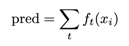
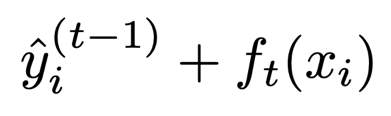
A note to the observant reader (not from the docs): In the above expansion, the loss functionwhere the independent variable is in the form
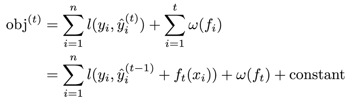
Mathematical Description of XGBoost Optimization
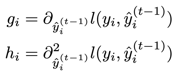
For the sake of making these equations more interpretable and concrete, assume we have a sample x such that the XGBoost model f outputs 0.2 = p = f(x), and assume we have a true label y = 1. The gradient of the logistic loss for this sample is g = p-y = -0.8. This will encourage the (t+1)st tree to be constructed so as to push the prediction value for this sample higher.
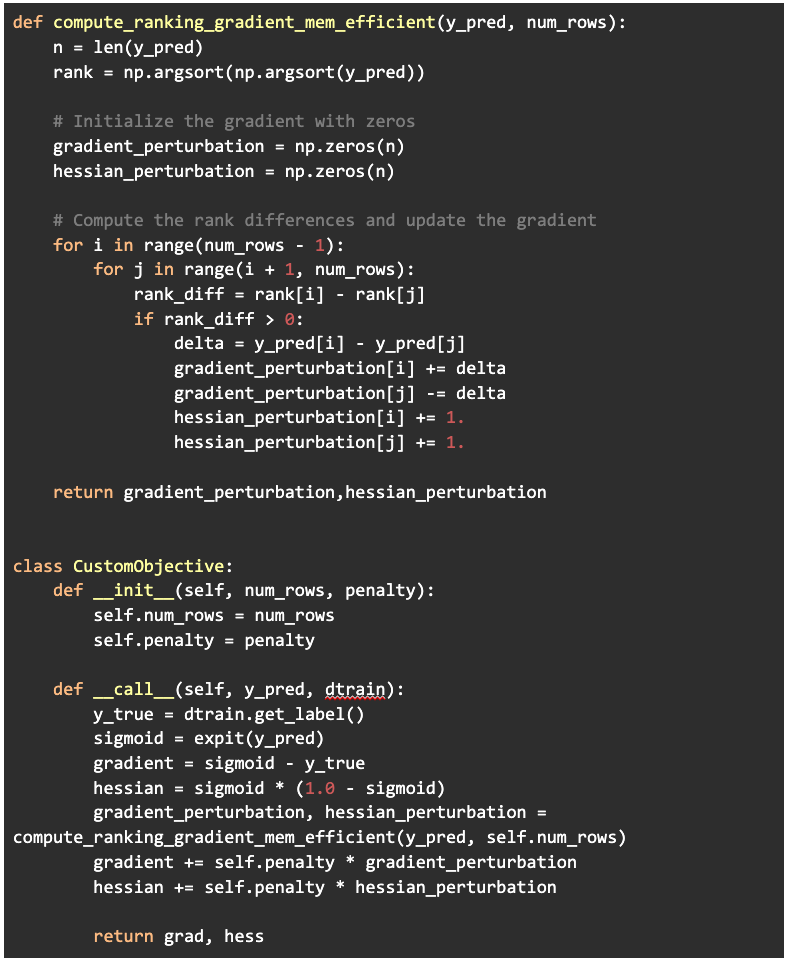
The perturbation value we decided to use was simply the difference between the pred values of each pair of misordered samples (ordered according to DV output by model N, or “old” model). Note that this requires a perturbation to the Hessian as well. This code assumes the values in the argument “y_pred” are ordered according to values output by model N. Take care to note that this does not mean these values are ordered as on the real number line. The scipy function expit is the sigmoid function with built-in underflow and overflow protection.

such that
and
The upshot is that if we want to customize the XGBoost objective, we need only provide the updated gradient gi and Hessian hi.
The upshot is that if we want to customize the XGBoost objective, we need only provide the updated gradient gi and Hessian hi.
respectively.
We ran two separate experiments, differing only in the number of training samples. The custom objective succeeded in reducing swap-in or “surprise” FPs with a minimal trade-off in true positives.
An Intuitive Toy Example
Experiments, Code, and Results
Experimental Setup
The takeaway is that a negative gradient pushes the prediction value and therefore the DV higher, as the sigmoid function is everywhere increasing. This means that if we want to customize the objective function in such a way that the DV of a given sample is pushed higher as subsequent trees are added, we should add a number v<0 to the gradient for that sample.
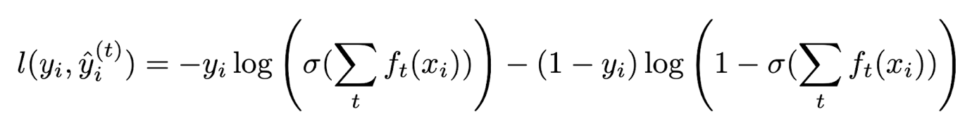
The objective function we leverage for training the binary classifier is the binary logistic loss function with complexity regularization
Results
| Comparison | Swap-Ins | Persistent FPS | Non-Swap New FPS | Total FPS Old Model | Total FPS New Model | Total TPS Old Model | Total TPS New Model |
| Old vs. Full | 32 | 194 | 23 | 226 | 250 | 25,267 | 28,111 |
| Old vs. Candidate | 26 (18.75%) | 199 | 25 | 226 | 250 | 25, 267 | 28,104 (0.025%) |
| Comparison | Swap-Ins | Persistent FPS | Non-Swap New FPS | Total FPS Old Model | Total FPS New Model | Total TPS Old Model | Total TPS New Model |
| Old vs. Full | 59 | 382 | 56 | 446 | 497 | 62,157 | 69,059 |
| Old vs. Candidate | 53 (10.2%) | 387 | 56 | 446 | 497 | 62,157 | 69,053 (0.009%) |
Python Implementation
Each experiment consists of training exactly three XGBoost binary classifier models on a set of 90/10 dirty/clean PE files. Featurization was performed with an internally developed static parser, but the method itself is agnostic to the parser. One could leverage the EMBER open-source parser, for example. The first model represents the “N” release trained with the standard XGBoost logistic loss objective. We call this the “old” model. The second model represents the standard “N+1” release trained with the same objective as the “old” model but with 10% more data and the same label balance. We call this the “full” model. The third model represents the candidate “N+1” release trained with the custom objective described above and on the same dataset as the “full” model.
The callable CustomObjective class instantiation is then passed to the standard xgb.train function. Incidentally, the callable class is another way, in addition to lambda functions, to pass additional arguments to Python functions called with a signature restriction on the number of arguments.
Employing an XGBoost Custom Objective Function Results in More Predictable Model Behavior with Fewer FPs
gives
CrowdStrike’s Research Investment Pays Off for Customers and the Cybersecurity Industry